An LLM Is Not the Program: What Is Actually Inside the Model File

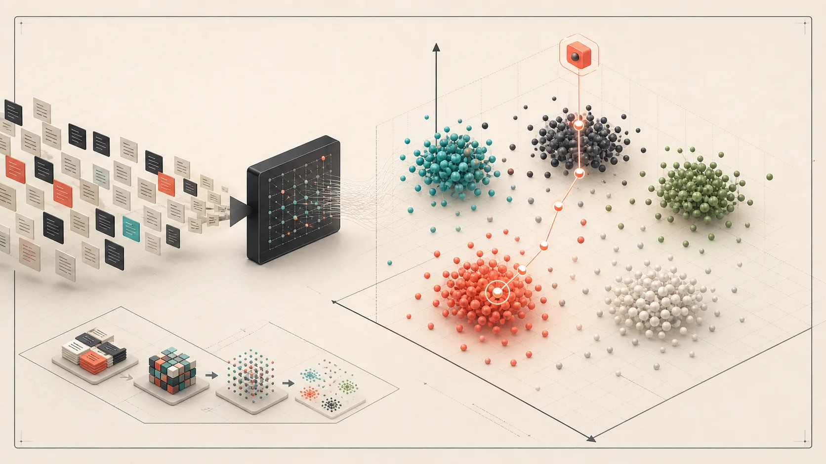
Part 1 of How LLMs Actually Run: from a familiar API call to tensors, parameters, and one transformer layer.

I understood how to call an LLM.

const response = await client.chat.completions.create({
  model: '...',
  messages: [...],
})

I understood the normal application concerns around that call: authentication, timeouts, retries, rate limits, streaming, structured output, and what to do when the provider returns something my code cannot use.

What I did not really understand was what happened after the API request arrived.

“The model runs” was doing an unreasonable amount of work in my mental model. What exactly is the model? Is it an executable? Is it a database? Where does its knowledge live? What does a GPU do with a 4 GB file full of numbers, and why does that eventually produce the token Paris?

The abstraction finally clicked when I stopped treating the model and the program running it as the same thing.

The first correction: the model is not really a program

When I run a local model with llama.cpp, two very different artifacts are involved:

llama.cpp  = executable code
GGUF       = model data

llama.cpp is native code. It knows how to read a model, tokenize input, construct computations, select CPU or GPU backends, manage inference state, and sample output tokens.

A GGUF file is mostly a large collection of learned numerical tensors plus the metadata required to interpret them. It does not contain a conventional implementation of answerQuestion() or a set of handwritten branches covering everything the model can say.

The runtime is the program. The model file is data the runtime knows how to execute.

That distinction sounds ordinary until you consider where the behavior lives. In traditional software, application behavior is mostly encoded in instructions written by engineers. Data drives those instructions, but we can usually point to the code that defines the decision.

With an LLM, an enormous amount of behavior is encoded in learned numerical relationships. The runtime supplies the stable algorithm. The model weights determine what that algorithm actually does with language.

This is not entirely foreign. A database engine is executable code while the database files hold the application’s records and indexes. A virtual machine executes bytecode produced elsewhere. A graphics engine applies general algorithms to scene data.

But an LLM pushes that separation much further. Change the weight file while keeping the runtime roughly the same, and vocabulary, style, factual associations, and capabilities can all change.

What a GGUF file actually contains

GGUF is a binary model format used by GGML-based inference runtimes. Its practical purpose is to package the information an executor needs to load and run a model efficiently, often as a single file.

At a useful level of abstraction, it contains:

• Metadata about the model and file
• The model architecture and its dimensions
• Tokenizer vocabulary and configuration
• Tensor names
• Tensor shapes
• Tensor data types and quantization formats
• Offsets locating each tensor in the binary data region
• The learned tensor values themselves

The GGUF specification describes a header, metadata key-value pairs, tensor descriptors, alignment padding, and the tensor data. That is enough for a loader to answer questions such as:

What architecture is this?
How many layers does it have?
Which tokenizer should interpret the prompt?
What shape is this tensor?
How are its values encoded?
At which byte offset do its values begin?

The tensor descriptors form what I think of as the tensor table. It is an index over the model’s large binary payload.

An abbreviated table might look conceptually like this:

name                       shape          type    offset
blk.0.attn_q.weight        [4096, 4096]   Q4_K    ...
blk.0.attn_k.weight        [4096, 1024]   Q4_K    ...
blk.0.attn_v.weight        [4096, 1024]   Q4_K    ...
blk.0.ffn_up.weight        [4096, 11008]  Q5_K    ...
blk.0.ffn_down.weight      [11008, 4096]  Q5_K    ...

The exact names and shapes vary by architecture. The important point is what the entries represent: learned transformations used at a particular location in the network.

The quantization type explains how the stored values have been compressed. Instead of storing every weight as a 32-bit floating-point value, a quantized model can represent groups of weights with far fewer bits plus scaling information. That reduces file size and memory traffic at the cost of some precision and additional decoding work.

Quantization is one reason a model with billions of parameters can fit on consumer hardware. Seven billion parameters stored at four bits each require roughly 3.5 GB for the raw values before format overhead, metadata, and other tensors. The same parameter count at 16 bits is roughly 14 GB.

There is no France -> Paris record

My database-trained instincts kept looking for the row.

If a model can complete “The capital of France is” with Paris, where is that fact stored?

Not like this:

key: France.capital
value: Paris

There is no tensor row I can query to retrieve the capital of France. The association is distributed across many learned numerical relationships: token embeddings, attention projections, MLP weights, and the transformations applied throughout the network.

That is why “the model is a database” is occasionally useful but ultimately misleading. A database is designed to preserve and retrieve explicit records. A language model learns statistical structure that lets it transform a token sequence into a probability distribution over what comes next.

Knowledge is present in the behavior of the system, not stored as a clean set of facts.

This also explains why model knowledge is difficult to update surgically. Updating one business record is normal database work. Changing one factual association inside a neural network without affecting related behavior is a much less local operation.

Parameters and weights are almost the same conversation

A parameter is a learned scalar value in the model. Weights make up the overwhelming majority of those values, though architectures may also include learned biases, normalization parameters, and other learned values.

Consider one weight matrix:

4096 × 4096 = 16,777,216 parameters

That is one matrix in one part of one layer. Add the attention projections, MLP projections, embeddings, output projection, normalization parameters, and many repeated layers, and billions of values arrive quickly.

This is what the 7B in “a 7B model” means: approximately seven billion learned parameters.

It does not mean seven billion facts, seven billion lines of code, or seven billion independent rules. It means the training process adjusted roughly seven billion scalar values.

More parameters can increase capability because they create more representational capacity:

• Wider hidden representations can preserve more features at once.
• Larger projection matrices can learn more transformations.
• Deeper networks can compose those transformations across more stages.
• Additional attention heads or larger intermediate dimensions can model more relationships.

But “more parameters means smarter” is not a reliable engineering rule.

Parameter count says nothing by itself about training data quality, architecture, optimization, tokenizer design, post-training, quantization damage, context handling, or inference strategy. A smaller model trained deliberately for a domain can outperform a larger general model on the work that matters. A badly trained large model is still badly trained.

Capacity creates room to learn. It does not guarantee what was learned or how reliably it can be used.

Unpacking one decoder transformer layer

The GGUF tensor table becomes easier to understand once I know what one layer is trying to do.

A modern decoder-only transformer varies in details by architecture, but a useful simplified layer looks like this:

input
  ↓
RMSNorm
  ↓
Q / K / V projections
  ↓
self-attention
  ↓
residual addition
  ↓
RMSNorm
  ↓
MLP
  ↓
residual addition

The layer has two primary responsibilities:

Attention gathers useful information from other tokens.

The MLP transforms the information accumulated so far.

Everything around those operations helps keep the representation stable and allows information to flow through many layers.

RMSNorm stabilizes the input

The token representation entering a layer is a vector of learned features. RMSNorm rescales that vector based on its root mean square magnitude. I think of it as putting the signal into a range the next learned transformations expect.

Normalization is not where the model retrieves facts. It is infrastructure for making a deep stack of numerical transformations trainable and executable without values drifting into unhelpful ranges.

Q, K, and V decide what to gather

Attention produces three projections from the current token representations:

• Query: what information is this position looking for?
• Key: what kind of information does each earlier position offer?
• Value: what information should be collected if that position is relevant?

Suppose the sequence is:

The database rejected the write because it was read-only.

When processing it, one attention head may produce a query that aligns strongly with a key associated with database. The corresponding value can carry information about that earlier token into the current representation.

The analogy is imperfect. There is no literal lookup request saying “resolve this pronoun.” Q, K, and V are vectors produced by learned matrix multiplications, and different heads can learn very different relationships. But “what I need, what you contain, and what you contribute” is a useful starting model.

Scaled dot-product attention is commonly written as:

QKᵀ measures how strongly queries align with keys. Scaling keeps those scores in a manageable range. Softmax turns them into weights. Multiplication by V creates a weighted combination of the information available from the relevant positions.

For autoregressive generation, masking prevents a token from attending to future tokens that do not exist yet.

The original Transformer paper introduced this attention form. Current decoder architectures have changed normalization, position encoding, attention grouping, activation functions, and other details, but this core relationship remains recognizable.

The MLP transforms what attention gathered

After attention collects context, the MLP applies learned projections and a nonlinear activation to each token position. If attention is communication between positions, the MLP is local computation over the resulting representation.

This part often contains some of the largest matrices in the layer. A hidden vector might be projected into a much wider intermediate representation, gated or activated, and projected back down.

The exact operation is architecture-specific, but the role is stable: turn the gathered features into a more useful representation for the next layer.

Residual connections preserve the running state

Attention and MLP outputs are added back to the layer input through residual connections. Each layer does not replace everything the previous layers knew. It contributes another transformation to the representation moving through the network.

After dozens of layers, the final representation at each position has been repeatedly normalized, projected, mixed with earlier-token information, transformed, and carried forward.

The output head then maps the final representation to one score per vocabulary token. Those scores are logits. They are not yet the selected answer; they are the inputs to the sampling strategy.

Most of the work is matrix multiplication

Once I followed one layer, the giant tensor file stopped looking arbitrary.

The runtime repeatedly does operations shaped like:

activation vector × learned weight matrix → new activation vector

During prompt processing, it performs those operations for many token positions. During generation, it performs them again for each new token. Attention adds matrix operations across positions, while the MLP adds large projections within each position.

This is why GPUs are so useful. The model is not asking the processor to follow millions of unpredictable branches. It is asking for an enormous number of similar multiply-and-accumulate operations over dense blocks of numerical data.

The request has now crossed the first important boundary:

API request
    ↓
token IDs
    ↓
model architecture + learned tensors
    ↓
repeated transformer layers
    ↓
logits for the next token

That tells me what must be computed. It still does not explain how llama.cpp loads a GGUF file, builds those operations, moves weights into GPU memory, and executes them quickly.

That is the next layer of the stack.

Continue with Part 2: From GGUF to GPU: How llama.cpp Actually Runs a Model.

Alternate titles for review

• What Is Actually Inside an LLM?
• The Model Is Data: Following an LLM Past the API
• From Parameters to Attention: The First Layer Beneath an LLM API
• Why You Will Never Find France -> Paris in a Model File