From GGUF to GPU: How llama.cpp Actually Runs a Model

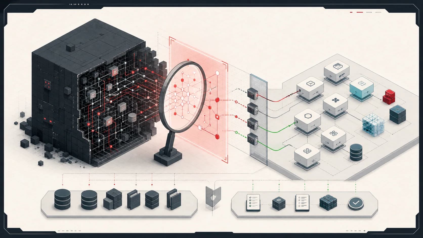
Part 2 of How LLMs Actually Run: from a GGUF tensor table through llama.cpp, CUDA, GPU memory, and one generated token.

In Part 1, I separated the model from the program running it. The GGUF file contains architecture metadata, tokenizer information, tensor descriptors, and billions of learned numerical values. llama.cpp is the executable that knows how to turn those values into transformer operations.

That fixed one abstraction leak and exposed another.

Saying “llama.cpp runs the tensors on the GPU” is directionally correct. It also skips almost every interesting engineering boundary.

How does a tensor at a byte offset inside a file become a matrix multiplication? Does the whole model move into GPU registers? What does llama_decode() actually do? And why can a consumer GPU perform this much work quickly enough to stream text back to a terminal?

The native-code flow

A deliberately abbreviated llama.cpp program looks like this:

model = llama_model_load_from_file("model.gguf", model_params);
ctx = llama_init_from_model(model, context_params);
tokens = tokenize(prompt);

llama_decode(ctx, batch);
logits = llama_get_logits(ctx);
next_token = sample(logits);

The current llama.cpp API contains these model-loading, context, decode, and logits operations. Real code needs backend initialization, vocabulary access, batches, token positions, error handling, sampling state, and cleanup. The short version is useful because it exposes the major responsibilities.

Load the model

llama_model_load_from_file() opens the GGUF file and interprets its metadata and tensor descriptors. It validates that the architecture is supported, creates tensor objects with the correct shapes and types, and arranges their storage according to the selected backends and model parameters.

Depending on the configuration, weights may remain mapped in system memory, be copied or offloaded to one or more GPUs, or be divided across devices. “Load the model” is therefore more than parsing a header. It establishes where the weight tensors will live and how later operations can access them.

Create the inference context

llama_init_from_model() creates runtime state around the loaded model.

The model and the context are deliberately separate concepts. The model owns the mostly immutable architecture and weights. The context owns state for an inference session: configured context size, batching information, compute buffers, and the memory used to avoid recomputing attention history.

This separation becomes important for concurrency. One set of model weights can serve many logical sequences, while each sequence retains its own state.

Tokenize the prompt

The tokenizer turns text into integer token IDs from the model’s vocabulary.

"A retry must be idempotent"
          ↓
[token_1, token_2, token_3, ...]

The model does not consume UTF-8 strings directly. It consumes token IDs, maps those IDs to learned embedding vectors, and then transforms those vectors through every layer.

Tokenization also explains why context length and output limits are measured in tokens rather than characters. The mapping is model-specific. The same string can become a different token sequence under a different tokenizer.

llama_decode() is where the model becomes computation

The most important call is llama_decode(ctx, batch).

Conceptually, it does four things:

1. Finds the embeddings and positions for the input tokens.
2. Builds the transformer operations required for this batch.
3. Executes those operations using the configured compute backend.
4. Updates inference state and makes output logits available.

The useful abstraction stack is:

llama.cpp
    ↓
GGML computation graph
    ↓
CUDA backend
    ↓
CUDA kernels
    ↓
GPU machine instructions
    ↓
VRAM / cache / shared memory / registers
    ↓
matrix operations

Each boundary answers a different question.

llama.cpp knows the model architecture: which tensor is the query projection for layer 12, which normalization occurs first, how rotary position information is applied, and how the residual path is assembled.

GGML represents the required tensor operations as a computation graph. The graph contains nodes for operations such as matrix multiplication, normalization, element-wise addition, activation, and attention-related transformations. It expresses what must be calculated and the dependencies between calculations.

The backend decides how to execute those graph nodes. A CPU backend uses optimized CPU routines. A CUDA backend selects or launches GPU implementations. Other supported backends can target different hardware without rewriting the model architecture as a new application.

CUDA kernels are functions executed by many GPU threads. They implement the actual work: loading tiles of tensor data, multiplying values, accumulating partial results, applying transformations, and writing outputs.

The compiler and GPU turn those kernels into machine instructions scheduled across streaming multiprocessors, CUDA cores, and Tensor Cores where applicable.

By the time I reach the bottom of the stack, “the model answered” has become a large sequence of loads, multiply-accumulate operations, synchronization, and stores.

The model does not live in GPU registers

This was one of my early misconceptions.

GPU registers are extremely fast, so I imagined the model being “loaded onto the GPU” as if billions of weights somehow sat next to the arithmetic units waiting to be used.

They do not fit there. The model primarily resides in VRAM, also called device or global memory in CUDA terminology.

Small working chunks move through faster, smaller memory structures while a kernel operates:

system RAM
   ↓ PCIe
VRAM / global memory
   ↓
L2 cache
   ↓
L1 cache / shared memory
   ↓
registers
   ↓
CUDA cores / Tensor Cores

This is a conceptual hierarchy, not a promise that every byte follows one identical route. Hardware generation, cache behavior, kernel design, unified memory, and backend choices complicate the details. The engineering constraint remains: capacity generally increases as we move upward in the diagram, while access becomes faster closer to the execution units.

VRAM holds the large persistent working set: model weights, activation buffers, KV-cache storage, and runtime workspaces. Registers hold values private to active threads. Shared memory is a programmer-managed on-chip region that threads in a block can use cooperatively. Caches reduce the cost of repeated global-memory access.

The CUDA Programming Guide describes these memory spaces and their relationship to threads and thread blocks. The practical takeaway for LLM inference is simple: moving data is part of the computation cost.

Matrix multiplication as a tiled data-movement problem

Imagine multiplying an activation matrix by a large weight matrix. The naive description is:

output = activations × weights

A useful GPU kernel cannot fetch every individual weight independently from VRAM, perform one operation, and forget it. The memory traffic would dominate.

Instead, kernels divide matrices into tiles. Threads cooperatively load useful blocks, reuse values across many multiply-accumulate operations, keep partial sums close to the execution units, and then write completed output tiles back to memory.

Tensor Cores accelerate supported matrix multiply-and-accumulate shapes and numerical formats. Quantized kernels add another concern: stored low-bit representations must be interpreted and scaled correctly while preserving enough throughput to justify the compression.

This is why backend and kernel quality matter. Two runtimes can execute the same weights and architecture while achieving different performance because one schedules work, moves data, or handles quantization more effectively.

The weights define the learned transformation. The kernel determines how efficiently the hardware performs it.

Prompt processing and token generation are different phases

An LLM request has two performance shapes that are easy to blur together.

During prompt processing, often called prefill, the runtime processes the provided token sequence. Many token positions are available at once, which exposes substantial parallel work. The runtime also records the attention keys and values that later tokens will need.

During generation, often called decode, the model produces one new token position at a time. That token can use the cached attention state for earlier positions, but it still needs to pass through the model’s layers.

prompt tokens
    ↓
full transformer pass over the prompt
    ↓
logits for the next position
    ↓
sample one token
    ↓
append it to the sequence
    ↓
run the transformer for the new position
    ↓
repeat

The model does not write the response privately and reveal it afterward. Autoregressive generation means the next token becomes part of the input used to produce the token after it.

Every generated token normally passes through every transformer layer. What makes generation practical is that the runtime does not recompute every earlier key and value from scratch. It keeps them in the KV cache.

Logits are not yet a token

After the final layer, the model produces logits: one score for each token in the output vocabulary.

The sampler turns those scores into a choice. It may apply temperature, top-k or top-p filtering, repetition controls, grammar constraints, or a deterministic greedy selection. Sampling strategy can materially change output even though the model weights are identical.

The chosen token is appended to the logical sequence, decoded into text when appropriate, and fed back into the next iteration.

Generation stops when the model produces an end-of-sequence token or the runtime reaches another stop condition, such as:

• A configured maximum token count
• A stop string or token sequence
• A grammar reaching a valid terminal state
• Client cancellation
• A context or resource limit
• A server timeout

The model can assign probability to an EOS token. The runtime still owns the surrounding lifecycle.

Why this is not impossibly slow

At this point the process sounds absurdly expensive. Billions of weights participate in repeated matrix operations for one token, and then the system does it again for the next token.

Why can a high-end consumer GPU generate tokens faster than some database requests return?

Because “expensive” and “hardware-hostile” are different properties.

LLM inference has:

• A huge amount of arithmetic
• Regular, predictable operations
• Dense numerical data
• Large blocks of parallel work
• Weights already resident in VRAM after loading
• Relatively few unpredictable control-flow decisions inside the core math

A database request can have far less arithmetic while paying for:

• Network round trips
• Pointer chasing through data structures
• Branch-heavy execution plans
• Cache misses
• Index traversal
• Locking or MVCC visibility checks
• Parsing and serialization
• Storage I/O when the working set is not cached

A database is optimized for selective access, transactional semantics, and changing records. An LLM forward pass is optimized around applying mostly fixed matrices to dense numerical state. The GPU is exceptionally good at the second workload.

The comparison is not “GPUs are faster than databases.” They are solving structurally different problems.

Generation often waits on memory bandwidth

Single-user token generation can be constrained more by memory bandwidth than raw arithmetic throughput.

For a small decode batch, the GPU may need to stream a large portion of the model weights from VRAM for each generated token while having limited opportunities to reuse each fetched value across many independent sequences. The arithmetic units can wait for data.

That is why quantization can improve speed as well as capacity: fewer bytes must move. It is also why headline FLOPS alone do not predict tokens per second. VRAM bandwidth, model size, quantization format, kernel quality, context length, batch size, and memory overhead all matter.

Add more active sequences to the batch, and the runtime can reuse weight reads across more useful work. That improves throughput—but requires a serving layer capable of keeping many independent sequences isolated and efficiently scheduled.

Continue with Part 3: One Model, Many Conversations.

Alternate titles for review

• What llama_decode() Actually Does
• From Model File to Matrix Math: Following llama.cpp Down the Stack
• Where an LLM Lives on a GPU
• Why Billions of Parameters Can Still Produce Tokens Quickly